LogNormとAsinhStretchで馬頭星雲を比較してみた｜Astropyで学ぶ画像伸張処理

エルシー(Elsy)

皆の者、ご機嫌麗しゅう！我は、生成AI猫 エルシーじゃ😊
マイペースだとよく言われるのじゃ!
出身地：Adobe Firefly（画像生成AI）

Hello everyone! I am Elsy, the AI-generated cat 😊
People often say I do things at my own pace!
Place of origin: Adobe Firefly (AI image generator)

オリバー(Oliver)

皆さん、初めまして！私は、オリバーです。
エルシーさんの助手猫です。
エルシーさんがよく暴走するので、暴走を止める役割をしています。
出身地：Adobe Firefly（画像生成AI）

Hello everyone! My name is Oliver.
I am Elsy’s helper cat.
Elsy sometimes gets out of control, so my job is to stop her.
Place of origin: Adobe Firefly (AI image generator)

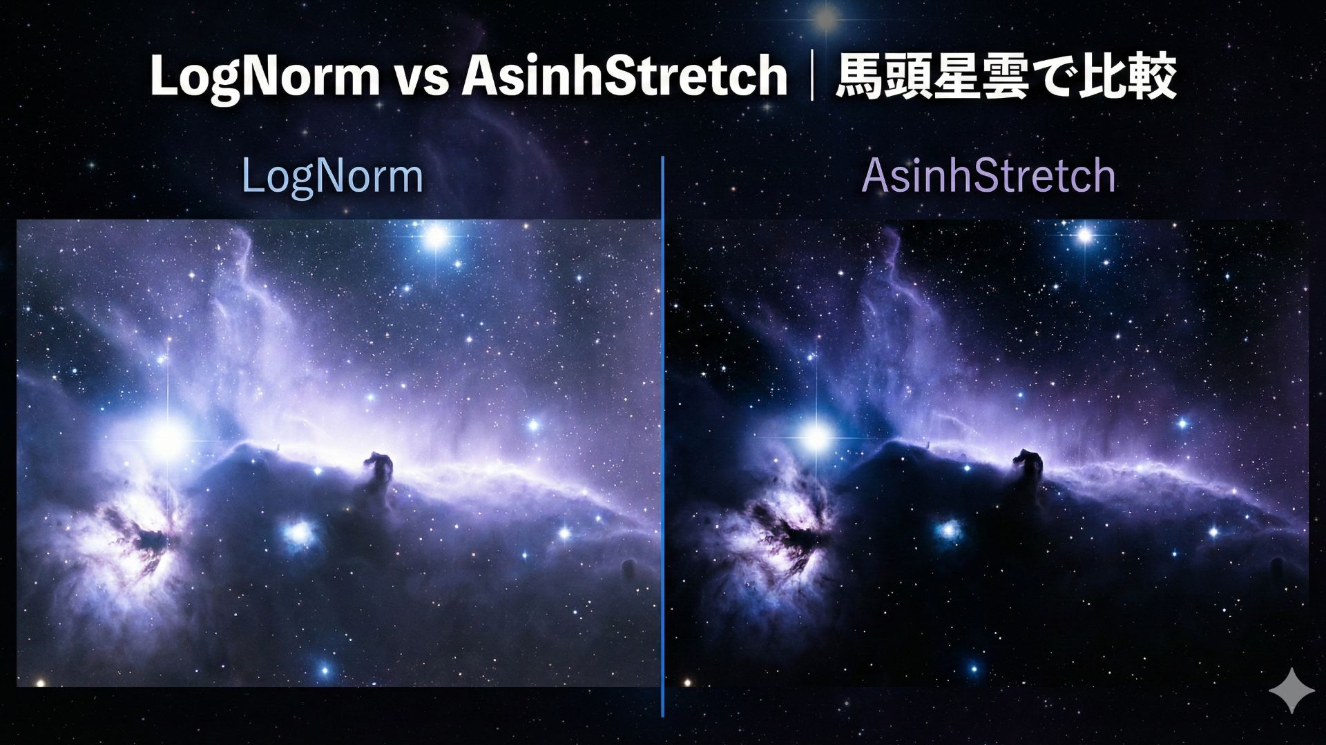
天体画像をより美しく、より正確に表現するためには「どの伸張処理を使うか」が重要です。本記事では、Astropyで利用できる LogNorm と AsinhStretch の2つの手法を使い、馬頭星雲（Horsehead Nebula）の画像を実際に比較しました。暗いガスの構造を強調したい場合や、明るい星の白飛びを抑えたい場合など、目的に応じた最適な処理方法が分かる内容になっています。初心者でも理解しやすいように、特徴・違い・実際のコード例を丁寧に解説します。

参考文献
公式サイト Astropy

Viewing and manipulating FITS images — FITS Images

learn.astropy.org

LogNormとAsinhStretchの違い

この２つの手法には、下記の違いがあるそうです！

• LogNorm: 全体的に明るくなりますが、中心部の明るい星のディテールが消えやすい。
• AsinhStretch: 暗いガスを浮かび上がらせつつ、中心部の星も白飛びせずに構造が見えやすい。

エルシー(Elsy)

暗い星雲を見つけたい場合は、LogNormを使うと良さそうなのじゃ！

オリバー(Oliver)

明るい星雲の構造をはっきり見たい場合は、AsinhStretchを使うのがいいですね！

馬頭星雲をLogNormで表示

馬頭星雲をLogNormで表示したのがこちらです。

import numpy as np

# Set up matplotlib
import matplotlib.pyplot as plt
%matplotlib inline
from astropy.io import fits
from astropy.utils.data import download_file
from matplotlib.colors import LogNorm

image_file = download_file(
    "http://data.astropy.org/tutorials/FITS-images/HorseHead.fits", cache=True
)

hdu_list = fits.open(image_file)
image_data = hdu_list[0].data

plt.imshow(image_data, cmap="gray", norm=LogNorm())


cbar = plt.colorbar(ticks=[5.0e3, 1.0e4, 2.0e4])
cbar.ax.set_yticklabels(["5,000", "10,000", "20,000"])
plt.savefig("LogNorm.png", format="png", dpi=300, bbox_inches='tight')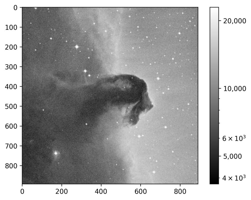

エルシー(Elsy)

綺麗な画像じゃが、中の構造がわかりにくいのじゃ！

馬頭星雲をAsinhStretchで表示

AsinhStretchを使って作成したのがこちらです。

import numpy as np
import matplotlib.pyplot as plt
%matplotlib inline
from astropy.io import fits
from astropy.utils.data import download_file

image_file = download_file(
    "http://data.astropy.org/tutorials/FITS-images/HorseHead.fits", cache=True
)

hdu_list = fits.open(image_file)
image_data = hdu_list[0].data

import matplotlib.pyplot as plt
from astropy.visualization import (ImageNormalize, AsinhStretch, 
                                   ZScaleInterval, PercentileInterval)

# 1. 正規化の設定を作成
# stretch に AsinhStretch を指定します
# interval で vmin, vmax を自動計算させると便利です（例：全体の99%をカバー）
norm = ImageNormalize(image_data, 
                      interval=PercentileInterval(99), 
                      stretch=AsinhStretch())

# 2. 画像の表示
plt.imshow(image_data, cmap="gray", norm=norm)
plt.colorbar(label='Intensity')
plt.savefig("AsinhStretch.png", format="png", dpi=300, bbox_inches='tight')
plt.show()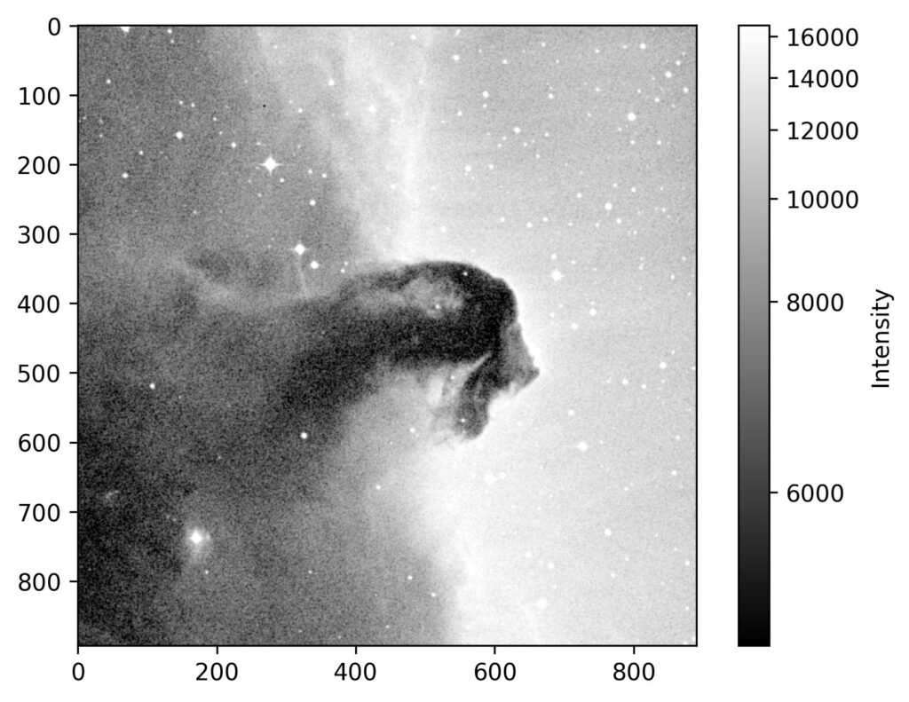

オリバー(Oliver)

AsinhStretchの方が全体的に白く見えています。

https://generative-ai-beginner-navi.com/